Kicking the Tires: Flatgeobuf
This week I’ve been out in the woods on an island at Gradient Retreat and it’s given me a chance to finally finish some research and experiments with Flatgeobuf, a new(ish) file format for storing geospatial vector data. In this post I’ll give a quick overview of the format and why I think it’s so interesting.
What is it?
Flatgeobuf is a binary data format for storing spatial vector data. It’s meant as an alternative to things like Shapefiles, KML, or GeoJSON, meaning you can store the usual sort of stuff from the OGC Feature Model (lines, polygons, etc) along with related properties.
But FGB includes a few optimizations that make it especially interesting:
- The use of flatbuffers for efficient feature / geometry encoding
- Inclusion of a built-in streamable spatial index as well as conventions around data layout to optimize remote retrieval using the index
Optimization 1: Flatbuffers for Efficient Geometry Encoding
Flatbuffers is a binary data serialization library. Similar to projects like Apache Thrift or Protocol Buffers, it provides an IDL for specifying data schemas along with implementations for reading these data types to and from bytes in a variety of languages
Like thrift or protobuf, there’s a code generator that turns your .fbs IDL specs into concrete implementations in your chosen language, as well as a runtime library which provides some of the serialization/deserialization machinery.
As a binary format, flatbuffers already has a leg up on text-based formats like GeoJSON or WKT in terms of data compactness and serde speed: you don’t have to repeat a bunch of field names as strings in your data and you don’t have to run through a text parsing routine to deserialize. But fbs also goes a step further than thrift or protobuf in that it’s designed for “zero copy” serde.
This means that the flatbuffers spec and associated runtime libraries go to great lengths to design memory layouts that can be used directly by host languages without having to first copy into a corresponding “language native” format.
For example in a library like thrift, you might have an internal convention for representing an Array of Ints in binary. This is better than something like JSON since it’s much faster to read a custom binary Array representation than a text-based one, but you still find that in order to actually use the data you’ll need to copy to a local representation like, say, java.util.ArrayList<Integer> . So you end up with 2 steps: first buffer the thrift/pbf-encoded data into memory from disk or network, then translate this binary data into language-specific representations.
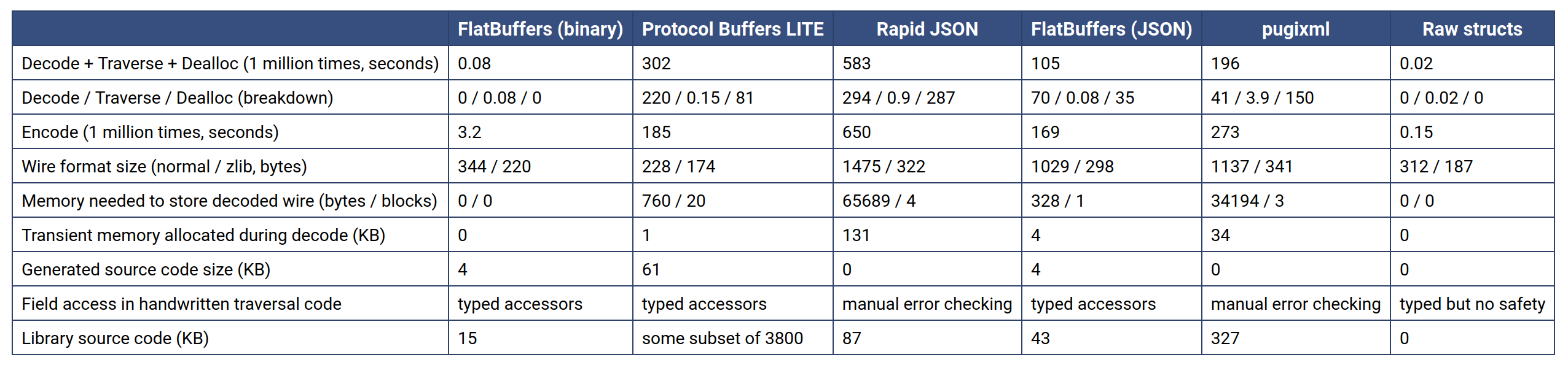
With flatbuffers, you skip the last step because the creators of the library have done binary magic to design memory layouts that can be used directly the same as other language-native datatypes. You can even read them directly from disk via mmap, etc. Of course, this tends to work best in languages like C++ or Rust which are used to giving you tight control over memory layouts, and it comes with a cost that the library can be complicated to use in comparison with thrift or protobuf (which already have their own non-trivial learning curve). But this is the price you pay to get sick sick serde speedups (you can see some related benchmarks here).
So the designers of Flatgeobuf decided to use this format for handling the encoding of feature geometries, which typically make up the bulk of a large vector dataset. As mentioned, this gives a lot of impact in particular on implementations in C++ or Rust, which is important since these versions often get integrated into other systems (e.g. using the C++ FGB implementation to add FGB handling to PostGIS or GDAL, or writing Python libraries which are just wrappers over native code implementations), so there’s a lot of leverage from this optimization.
Optimization 2: Streamable Hilbert-sorted RTree Index
The second exciting piece of flatgeobuf, and honestly what makes the whole thing worth the price of admission alone, is its approach to indexing. Including a pre-built index with geospatial data isn’t new — Shapefile and Geopackage support this, and there’s always spatialite if you want to pack your data into a sqlite file.
However flatgeobuf’s indexing and layout strategy is uniquely optimized for remote reading, i.e. consuming both the data and index piecemeal over the network, via HTTP requests. It targets the use case of “dump these files on S3 and read them directly from a client”.
To do this, the format combines an RTree index (the trusty workhorse of all geospatial indexing) with a compact and streamable encoding and a particular spatial ordering of the geometry data (using a Hilbert Curve) to make the whole thing more efficient. Here’s how it works.
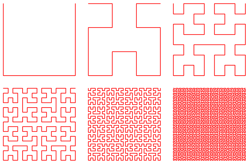
To write an indexed FGB file, you first sort your feature data along a Hilbert Curve. Space Filling Curves are a fascinating and brain-melting topic that merit a full post on their own, but in short they allow a linear encoding of multiple dimensions into 1 dimension (in our case, sorting a 2-dimensional xy space along a 1-dimensional curve). This is an optimization used in many spatial indexing systems to ensure that data with high storage locality also has high spatial locality.
In flatgeobuf, the feature data is stored in a long buffer containing back-to-back Flatbuffers of encoded feature geometries + properties, and these features are hilbert-sorted before being indexed and written to allow for more efficient I/O batching when looking data up via the index.
Side Note: There’s a lot of research on different methodologies for spatial sorting for indexing. Flatgeobuf uses the Hilbert encoding of the center of each feature’s bounding box, referred to as “2D-C” in the literature. (https://dl.acm.org/doi/10.1145/170088.170403).
Next, a “packed” RTree is built to represent these nodes, where “packed” means that the tree is maximally filled (no empty internal slots), which is possible since we are building it in bulk from a known static dataset (FGB is not aimed at supporting updates in place).
The tree is built “bottom-up”, with the pre-sorted features making up the bottom layer. For this layer you construct a vector of Index Nodes containing a bounding box for the feature and its byte offset in the data section of the overall file.
Then a tree is built by adding upper layers of internal nodes as needed, with each internal node’s bounding box representing the superset of all its children’s bounding boxes, and its byte offset pointing to the location in the index buffer where its list of child nodes begin.
Once the tree reduces down to a single root node, it is flattened out for storage with each layer stored sequentially one after the other.
Here’s a diagram showing an example tree. Note that since the tree is fully “packed”, its structure is determined purely by the number of features and node size (branching factor). For 4 features with a node size of 2 we get this:
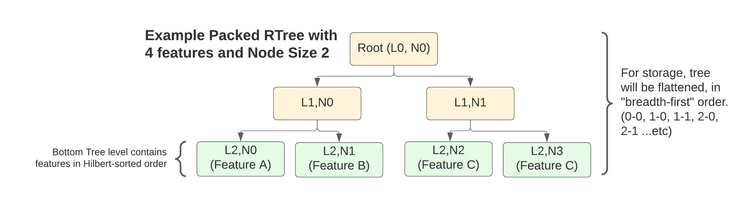 FGB RTree Index Layout Example
And here’s how that tree would be serialized into the final FGB file:
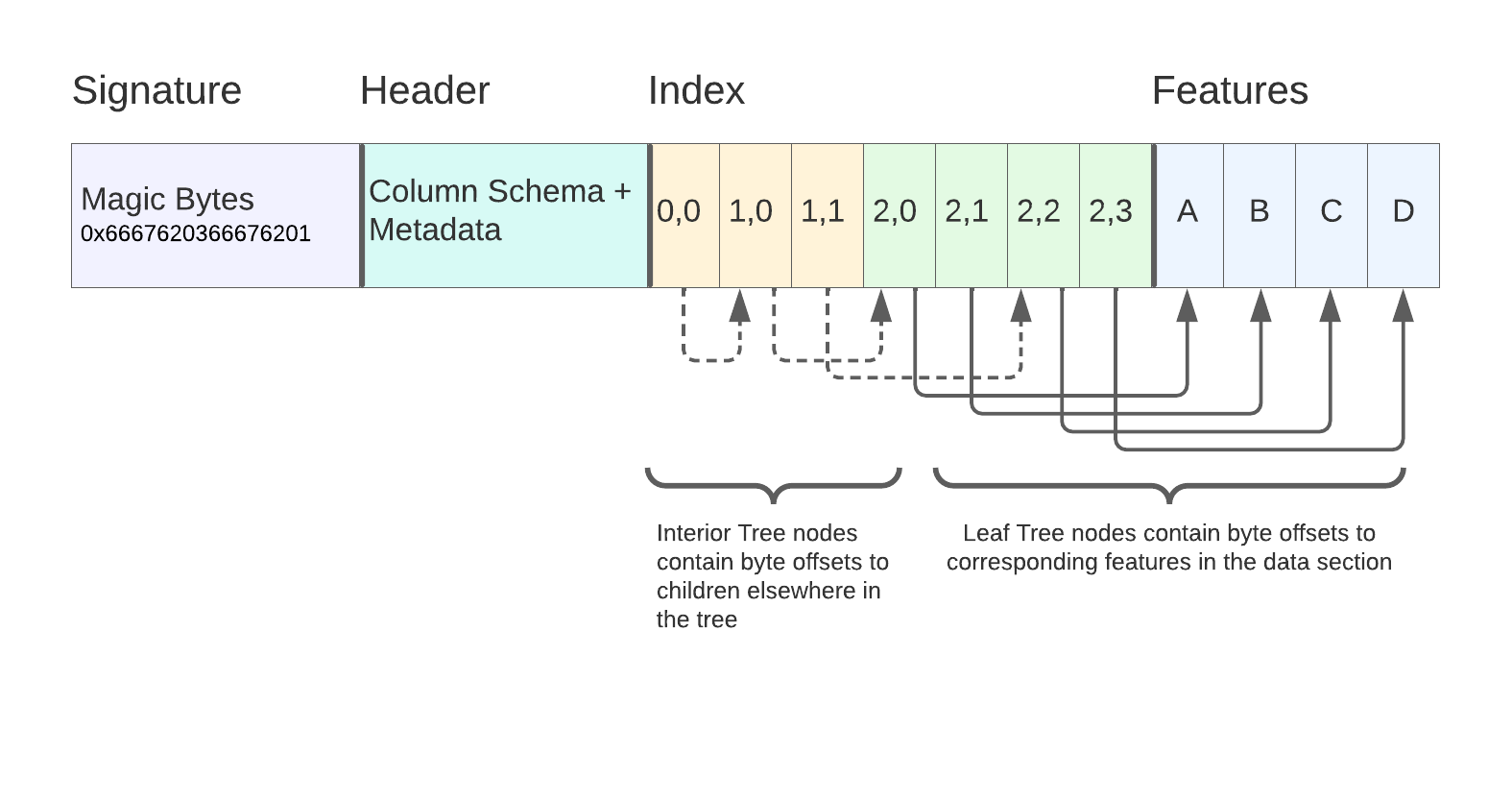 FGB file layout after flattening tree
Indexing Takeaways: Cloud-native GIS Vector Data
That’s a lot of detail about how the indexes are put together, but what does it actually mean?
The point is that both the index and the underlying feature data are designed to be loaded lazily — a client can stream the portions of the index they need to satisfy a bounding-box query, then use those results to stream the relevant portions of the Feature section. This can all be done either locally (reading from a potentially large file) or remotely over HTTP using Range requests.
This means you can literally chuck an FGB file on S3 and serve it directly to clients, without any persistent server process in the mix. It’s a piece of “serverless” tech which isn’t just marketing vapor-speak, and it has the potential to open a lot of new architectural patterns for managing Geospatial data.
To quote Brandon Liu:
A Map is just a Video
And formats like FGB drive that home: the way these cloud-native GIS formats incrementally pull data from remote storage is the same way that streaming video codecs lazily pull the next frames in your favorite Netflix movie. Panning around a slippy map is like scrubbing forward and backward through a video of the earth.
Here’s a demo on the flatgeobuf.org site that shows this in action: live slippy map filtering of a 12GB US Census Block dataset direct from storage over HTTP
 leaflet Census Block filtering demo](/public/images/fgb_slippy_demo.png) flatgeobuf census blocks slippy map demo
flatgeobuf census blocks slippy map demo
I’m particularly hopeful about the potential to bridge the gap between offline “big data” use-cases, which want to consume static files from cloud storage, and online interactive use-cases like a simple slippy map viewer. Traditionally, the latter required an indexed server process like PostGIS, but now you might be able to have both of these systems reading from the same static cloud-storage-hosted datasets.
Downsides?
- Complexity — No denying the format is pretty complicated. Between sophisticated binary encodings and optimized indexing strategies there is a lot going on in these bytes. Small errors in encoding or indexing can render files unreadable. To become more mainstream, the format will need better linting tools to validate structural correctness of without a lot of painful
hexdump-ing. - Not human readable — Especially compared to simpler formats like GeoJSON and WKT this is always a downside. Of course the benefits are huge (smaller storage footprint, faster serde), but it will take really polished tooling to ease people off of text-based formats. On the other hand Shapefiles aren’t human-readable and ESRI has managed to jam those down everyone’s throats for several decades, so maybe there’s hope.
- Not designed for updates — Because of the intricacies of data layout and indexing, updates aren’t really a thing for FGB. It’s best used for static datasets.
- Non-spatial indexing — Currently the format doesn’t really have a way to add indexing on other dimensions besides the spatial one. Maybe this will evolve in the future (FGB’s first sidecar?)
Further Reading / Prior Art
- Big thank you to Björn Harrtell for designing this cool format
- Flatbush and Geobuf, JS libraries from Vladimir Agafonkin inspired the Hilbert-sorted RTree indexing and binary format for Flatgeobuf
- rawrunprotected/hilbert_curves: Provides a very cool algorithm for fast encoding of X,Y values to Hilbert numbers used by many of these libraries. This in turn appears to be partially inspired by a similar algorithm in Hacker’s Delight, Chapter 16.
- RTree packing + Hilbert Sorting: There’s quite a lot of academic literature about this, focusing on different strategies for bulk-loading RTrees and different sorting approaches to optimize lookup locality. These 2 articles are a good starting point:
- Direct spatial search on pictorial databases using packed R-trees, Roussopoulos & Leifker
- On packing R-trees, Kamel & Faloustos
- Cloud Optimized GeoTIFF: Another data format that has been bringing similar benefits to geospatial Raster data.
Where to go next?
- https://github.com/flatgeobuf/flatgeobuf for official support, including drivers for Rust, C++, JS, Java, and C#
- https://github.com/worace/geoq - My own Rust-based GIS CLI now has a
fgbsubcommand (version 0.0.21 — hot off the press) for reading and writing flatgeobuf files from GeoJSON at the command-line –echo '{"type": "Point", "coordinates": [0,0]}' | geoq fgb write /tmp/myfirst.fgb - As part of writing this article I went through the exercise of writing my own fgb writer implementation. I plan to publish a more detailed “implementer’s guide” focusing on the nuances of the spec based on what I learned from this experience.