Flatgeobuf: Implementer's Guide

Recently I went through the exercise of writing a flatgeobuf writer implementation, partly to add support for it to geoq and partly to help myself understand the format more thoroughly. Here are some notes based on my experience, covering some of the questions I had about the spec and which I had to refer to the existing reference implementations to answer.
This isn’t a spec per se but may be a helpful reference for anyone else trying to understand how an FGB file works, or implementing their own version. If you’re not deep in the weeds of trying to implement or understand the FGB encoding, you may find a previous post more useful as an oveview: Kicking the Tires: Flatgeobuf.
FGB File Structure
A flatgeobuf file is a binary data file made up of 4 parts:
- File Signature: 8 “magic bytes” indicating the file type and spec version
- Header: A length-prefixed flatbuffer containing a Header record from the
FlatGeobuffbs namespace. - Index (optional): A flattened, packed RTree containing a spatial index for performing bounding-box filtering of Features in the subsequent Data section. If the index is omitted this is indicated by setting the
index_node_sizeHeader field to0, and in this case the Features section will appear immediately after the Header. - Features / Data: A buffer containing sequential length-prefixed Feature flatbuffer records.
Here’s a diagram from the flatgeobuf site showing the full file layout:

In the rest of this post I’ll go through these sections giving more detail on each.
Note on Binary Encodings
Here are 2 conventions used for encoding binary data in these files:
- Flatbuffer records are used in several places, and they are always “size-prefixed”, meaning that each byte buffer includes 4 initial bytes to indicate the remaining size. The API for this varies a bit between languages, but they should be written with
finish_size_prefixedor the equivalent. - In a few cases numbers or other data are written to binary directly, outside of Flatbuffer records, and in these cases little-endian encodings are used. (e.g. f64.to_le_bytes in Rust)
Signature / Magic Bytes
The first 8 bytes of a fgb file are a signature, containing: ASCII F , G, B, followed by the spec major version (currently 03), then F,G,B again, then the spec patch version (currently 01).
So altogether this looks like:
// Rust example
vec![0x66, 0x67, 0x62, 0x03, 0x66, 0x67, 0x62, 0x01];
Or just 0x6667620366676201 in Hex.
Header
The header contains general metadata about the file, including properties schema, information about the index, etc. Note that some of the data included in the header requires either making a pass through the feature data, or having it statically provided as configuration (e.g. to calculate the number of features or dynamically infer the properties schema). More on this in the Indexing section.
Here are the header fields from the spec with some notes on what they mean.
name- String - arbitrary name given to your file. Many implementations will include this as a FeatureCollection-level property when converting to GeoJSONenvelope: f64/double array - 4 element bounding box encoded asminX,minY,maxX,maxYgeometry_type:GeometryTypeflatbuffer enum describing which geometry type appears in the file. If your FGB file only contains 1 type of geometry, you can specify it here. If the file is heterogeneous w/r/t geometry type, the header should specify geometry typeUnknownand then each individual Feature should specify their own geometry type.has_z: boolean - True if geometries in your file have Z coordinates. Note that additional coordinate dimensions are “all or nothing” for a geometry because they are stored in a separate vector. So if you want to support z for even a few points, you need to populate these vectors with 0’s for the remaining pointshas_m,has_t,has_tm- same ashas_z
columns: Array of flatbuffer Columns. This represents the properties schema for your file. By default, flatgeobuf assumes a heterogeneous schema for your features, i.e. that each feature has the same set of properties, or at least that the set listed here covers the superset of all used properties (individual features can skip a property from this list if they don’t have it). You can see the list of available column types in the spec.features_count: ulong (64bit unsigned int) - Number of features in the dataset. This has to either be provided as an argument or (more commonly) be calculated by first making a pass through all of the feature data before generating the headerindex_node_size: ushort (16-bit unsigned int) - default 16 - This represents the branching factor of the RTree used for the flatgeobuf spatial index, i.e. the number of child nodes under each interior node in the tree. Higher branching factor = wider, shorter tree. Obviously this can impact the size of your tree and the performance of your index lookups but the exact characteristics will depend on your dataset.crs: Crs - custom flatbuffer type - Specifies the CRS for the dataset. Most commonly this will be an org/code pair likeorg: EPSG, code: 4326title,description- Arbitrary strings for dataset description. No clear convention in how these are used in most implementationsmetadata: string, but expected to encode an arbitrary JSON object containing key/value metadata about the dataset
Heterogeneous vs Homogeneous FGB files
FGB supports heterogeneous or homogeneous files with regard to:
- Geometry Type
- Feature properties schema, i.e.
columns
In the case of a homogeneous collection (a file that contains 1 single type of geometry, or 1 consistent properties schema for every feature), these fields will be set in the Header so that they can be omitted in the individual Feature records. This saves space since the same schema information doesn’t have to be repeated in every feature.
In the case of a heterogeneous collection, they can be set in the individual features. For Geometry type, a special type of Unknown is used in the Header to indicate this.
Features Buffer
Technically the Index section comes next in terms of File order, but I’m going to start with the Features section since it sets the groundwork for the indexing.
The Features or “Data” section of the FGB file contains the bulk of the actual information. These are Features in the “OGC” sense, meaning a combination of a Vector Geometry and some set of properties.
The Geometry is encoded using its own Flatbuffer record type, while the properties use a custom binary encoding.
Here is the Feature schema:
table Feature {
  geometry: Geometry;  // Geometry
  properties: [ubyte]; // Custom buffer, variable length collection of key/value pairs (key=ushort)
  columns: [Column];   // Attribute columns schema (optional)
}
To serialize features, translate them into this encoding, then use the Flatbuffers API to write the record to a size-prefixed byte buffer. The Features section of the file simply contains a series of these buffers back to back.
Geometry Encoding
table Geometry {
  ends: [uint];          // Array of end index in flat coordinates per geometry part
  xy: [double];          // Flat x and y coordinate array (flat pairs)
  z: [double];           // Flat z height array
  m: [double];           // Flat m measurement array
  t: [double];           // Flat t geodetic decimal year time array
  tm: [ulong];           // Flat tm time nanosecond measurement array
  type: GeometryType;    // Type of geometry (only relevant for elements in heterogeneous collection types)
  parts: [Geometry];     // Array of parts (for heterogeneous collection types)
}
In the interest of compactness and type consistency the Geometry encoding avoids nesting in favor of flattened arrays that are zipped together at read-time. XY coordinates are encoded together in a single alternating vector (even indices are X’s and odds are Y’s).
The ends field indicates stop-coordinate positions to divide individual rings or segments in the case of Polygon and MultiLineString geometries, meaning it’s a Vec<f64> with a list of dividers rather than Vec<Vec<Vec<f64>>>.
Higher coordinate dimensions are optional and if used have their own separate vectors that align by index with the corresponding xy pairs.
This is easier to show rather than explain so here are some worked examples of different Geometry types, from GeoJSON to FGB.
Point
{"type":"Point","coordinates":[1,2,3]}
Geometry {
  xy: [1,2],
  z: [3],
  type: 1
}
LineString
{"type":"LineString","coordinates":[[1,2,3],[4,5,6]]}
Geometry {
  xy: [1,2,4,5]
  z: [3,6],
  type: 2
}
Polygon
Polygon (1 ring, shell-only)
- For shell-only polygon,
endsis unused - XY contains flat list of all coordinates
{
  "type": "Polygon",
  "coordinates": [
    [
      [-118.4765625,33.92578125],
      [-118.125, 33.92578125],
      [-118.125, 34.1015625],
      [-118.4765625, 34.1015625],
      [-118.4765625, 33.92578125]
    ]
  ]
}
Geometry {
  // All coordinates from the ring flattened
  // First coordinate is still repeated to close the ring as in WKT/GeoJSON/etc
  xy: [-118.4765625,33.92578125,-118.125,33.92578125,-118.125,34.1015625,-118.4765625,34.1015625,-118.4765625,33.92578125]
  type: 3
}
Polygon (1 outer, 1 inner ring)
endsare the cumulative coordinate number (1-indexed, i.e. the vector length) of the final coordinate from each ring. So a 4-sided polygon with 1 4-sided inner ring has 2 ends, first at 5 (5 coordinates for the outer ring) then at 10 (5 more coordinates for the inner ring, so the inner ring ends at coordinate number 10)
{
  "type": "Polygon",
  "coordinates": [
    [
      [-118.4765625,33.92578125],
      [-118.125, 33.92578125],
      [-118.125, 34.1015625],
      [-118.4765625, 34.1015625],
      [-118.4765625, 33.92578125]
    ],
    [
      [-118.24447631835938, 34.0521240234375],
      [-118.24310302734375, 34.0521240234375],
      [-118.24310302734375, 34.053497314453125],
      [-118.24447631835938, 34.053497314453125],
      [-118.24447631835938, 34.0521240234375]
    ]
  ]
}
Geometry {
  // all coordinates from BOTH rings flattened
  xy: [-118.4765625,33.92578125,-118.125,33.92578125,-118.125,34.1015625,-118.4765625,34.1015625,-118.4765625,33.92578125,-118.24447631835938,34.0521240234375,-118.24310302734375,34.0521240234375,-118.24310302734375,34.053497314453125,-118.24447631835938,34.053497314453125,-118.24447631835938,34.0521240234375]
  ends: [5,10], // 1-indexed coordinate number for last point per ring
  type: 3
}
Similar/Re-used encodings
These 2 are structurally the same as previous ones, so they use the same representation with a different type
- MultiPoint is encoded like LineString
- MultiLineString is encoded like Polygon
Collection Types
MultiPolygon and GeometryCollection make use of the parts field. The sub-geometries are encoded using the previous rules, then inserted into the parts vector. The top-level coordinate fields are unused.
Future Types
So far I’ve only researched and implemented the FGB geometry types that correspond to GeoJSON geometry types. Hopefully I’ll expand to cover the remaining ones in future. I’m not actually sure if any of the existing FGB implementations cover these types. It’s possible the C++/GDAL one does.
CircularString = 8,
CompoundCurve = 9,
CurvePolygon = 10,
MultiCurve = 11,
MultiSurface = 12,
Curve = 13,
Surface = 14,
PolyhedralSurface = 15,
TIN = 16,
Triangle = 17
Feature Property Encoding
FGB encodes Feature properties using a custom binary representation. In the Flatbuffer schema this appears as:
properties: [ubyte]; // Custom buffer, variable length collection of key/value pairs (key=ushort)
Meaning it’s just a byte vector embedded within the Flatbuffer record. This encoding is a compromise due to the challenges with representing highly polymorphic collections using Flatbuffers. It’s a tightly optimized format but this comes with some constraints, and to achieve the level of flexibility required here the designers decided to use a custom representation rather than lean on a Flatbuffer one.
Properties Schema Representation (Columns and ColumnTypes)
Property Schemas in FGB are represented as a vector of Column records. These are stored either in the Header (when the same schema is used across all features):
table Header {
  columns: [Column];
  // truncated...
}
Or in a Feature (if a custom schema per feature is needed):
table Feature {
  columns: [Column];
}
A Column represents a single property field, like so:
enum ColumnType: ubyte {
  Byte,                         // Signed 8-bit integer
  UByte,                        // Unsigned 8-bit integer
  Bool,                         // Boolean
  Short,                        // Signed 16-bit integer
  UShort,                       // Unsigned 16-bit integer
  Int,                          // Signed 32-bit integer
  UInt,                         // Unsigned 32-bit integer
  Long,                         // Signed 64-bit integer
  ULong,                        // Unsigned 64-bit integer
  Float,                        // Single precision floating point number
  Double,                       // Double precision floating point number
  String,                       // UTF8 string
  Json,                         // General JSON type intended to be application specific
  DateTime,                     // ISO 8601 date time
  Binary                        // General binary type intended to be application specific
}

table Column {
  name: string (required);      // Column name
  type: ColumnType;             // Column type
  title: string;                // Column title
  description: string;          // Column description (intended for free form long text)
  width: int = -1;              // Column values expected width (-1 = unknown) (currently only used to indicate the number of characters in strings)
  precision: int = -1;          // Column values expected precision (-1 = unknown) as defined by SQL
  scale: int = -1;              // Column values expected scale (-1 = unknown) as defined by SQL
  nullable: bool = true;        // Column values expected nullability
  unique: bool = false;         // Column values expected uniqueness
  primary_key: bool = false;    // Indicates this column has been (part of) a primary key
  metadata: string;             // Column metadata (intended to be application specific and suggested to be structured fx. JSON)
}
As of today, many of these Column fields aren’t used or may be implementation-dependent. name and type are the most important.
Since the Columns contain the field names, the combination of Column vector + individual feature properties can be used to derive a name → value map for each Feature (for example if converting to a GeoJSON properties JSON object).
Per-property encoding
Once the schema is established, encode individual properties as a byte buffer containing a sequence of:
u16(2 bytes) column indices — this indicates the “key”, by way of pointing to the index of the appropriate column in the Columns vector- Appropriate per-type binary representation (covered below). Depending on the ColumnType, sometimes these are statically sized and sometimes they include a length prefix. So for a
Boolcolumn it will always be 3 bytes — 2 for the index and 1 for the bool itself (u8, little-endian). For a String, it’s variable, with 2 bytes for the column index, then a 4-byte unsigned length, then a UTF-8 encoding of the String.
‼️ Note on field heterogeneity - I don’t know if the spec explicitly states this, but it’s probably bad to repeat Column names in a schema. Technically the structure (since it’s a Vector and not a Map) could model encodings where the same field name appears multiple times with a different ColumnType. But this will probably be highly implementation-dependent.
Column Type Binary Representations
- Numeric Types (Byte — Double) - These are all fixed size (size is known based on the type, so they’re encoded as 2 bytes for column index + 1–8 bytes for the appropriate little-endian data.
- String + Json - These are both written as UTF-8 Strings (Json is just an application-specific indication to use a String to contain serialized JSON data). So they are written as 2 bytes for index, 4 bytes for length, and N bytes for data.
To encode the full properties for a feature, write all of the individual columns back-to-back into a byte buffer, and use this to populate the [ubyte] properties field. As far as I know there is not a requirement around ordering of properties within a single feature.
Once you have all this assembled (Geometry + Properties + Columns if needed), serialize it using the flatbuffers size-prefixed binary encoding.
Feature Ordering (Hilbert Sort)
That covers how Features are represented individually, but not how they are ordered. As an optimization to improve Indexing, FGB sorts Features based on a Hilbert encoding of their geometric centers. This technique is used in many spatial indexing systems to improve data locality for records that have high spatial locality. The heuristic isn’t perfect in all cases, but especially for I/O Bound systems, it can help minimize the number of disk pages (or HTTP requests) required to satisfy a given spatial query (with Bounding Box queries being the most common).
There are a lot of details around the specific Hilbert-sort used by FGB, so it’s hard to describe in a concrete “spec”. It largely comes down to matching the behavior of a reference implementation, such as the official C++ implementation.
The code snippet for doing the actual Hilbert encoding was originally taken from this project. The use of this technique was heavily inspired by Vladimir Agafonkin’s flatbush library.
So, follow a reference implementation for the details, but here’s a rough description of how FGB Hilbert-sorts Features:
- Find the centroid of the feature geometry (X,Y only)
- Encode it to a single unsigned 32-bit Hilbert int using the reference algorithm
- (Aside: I’ve wondered if there is a name for this algorithm. The book Hacker’s Delight describes a similar algorithm as a “non-recursive algorithm for generating the Hilbert Curve”, so maybe that’s a start)
- Sort features according to those numbers
- Write these sorted, size-prefixed flatbuffers into the “Data” section of the final FGB File.
- Important: As the features are written, each one’s Bounding Box and Byte Offset within the Data section must be recorded. These Bounding Box + Byte Offset pairs are used to build the bottom layer of the RTree which makes up an FGB index, which we’ll look at next. This is why in most implementations Feature writing comes first, even though they actually come after the Index in the final output file.
❓ Note on Unindexed FGBs: As mentioned in the “File Layout” section, the Index in FGB is optional. The spec isn’t entirely clear on whether the Hilbert-ordering is expected in an unindexed file. Technically it shouldn’t matter (the purpose of the Hilbert-ordering is to optimize the index) but this may end up being application-specific.
Indexing
So now we’ve written a byte buffer of back-to-back size-prefixed flatbuffer Feature records which are ordered by a centroid Hilbert encoding, and recorded the byte offsets and bounding boxes for each of those features.
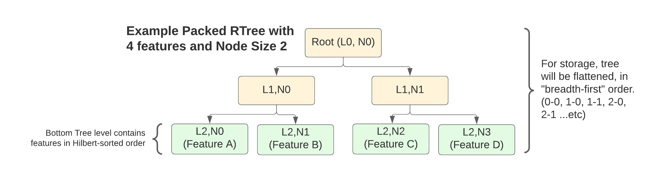
The index starts with these BBox + Offset “Index Nodes” forming the bottom layer of a Packed R-Tree. Because the tree is built in bulk from a static dataset, and it is “packed” meaning no empty internal spaces are left, the structure of the tree is fully determined by number of features and the node size or branching factor (this is the index_node_size field from the Header)
Basically, you lay out a bottom layer of all the Feature-representing index nodes pulled from writing that section:
// Bytes 0, 502, and 1029 would be the starting point of these respective Features
// in the previously written Data section. They allow consumers of the file
// to skip to the appropriate read position after consulting the index to
// find a Feature matching a given Bounding Box query
|Byte: 0, BBox:x1y1x2y2|Byte:502: BBox:x1y1x2y2|Byte: 1029, x1y1x2y2|
Then stack as many layers of “interior” nodes on top of these as required to build the tree up to a single root node.
For the Interior Nodes, the structure is the same (BBox + Byte Offset). However for these nodes, the Byte Offset points to the location of that node’s first child within the tree. This location can be known in advance because the size of each node is fixed and the structure is derived from the number of features + the index node size.
Finally, all of this gets written to a flattened byte buffer layer by layer, starting from the Root.
Note that my descriptions of stacking tree layers on top of one another are more about the conceptual structure of the tree, since it’s actual encoding is “flat”…it’s modeled in memory via skipping around in a single byte buffer rather than storing a graph of pointers.
Index Node Binary Encoding
Similar to properties, the tree index nodes use a custom binary encoding, but it’s fairly simple:
- 4 little-endian Doubles for the bounding box (minX, minY, maxX, maxY)
- Byte Offset: 64-bit unsigned int
For a total of 40 bytes per node.
So, to give a worked example, consider a FGB file with:
- 179 features
- Index Node Size (branching factor) 16
You would end up with:
- 3-level tree, with 1 node in the first (root), 12 nodes in the second, and 179 nodes in the last level (representing the actual features)
- 192 total nodes
- 7680 total bytes for the index
As mentioned, the node size is configurable, and can be used to make wider or narrower index trees. I’m not aware of any published analysis on this, but presumably it can have a big impact on how the index performs on different datasets.
Full File Layout Diagram
So, with all these pieces in mind, here’s a diagram of what a complete FGB file looks like (obviously not to scale).
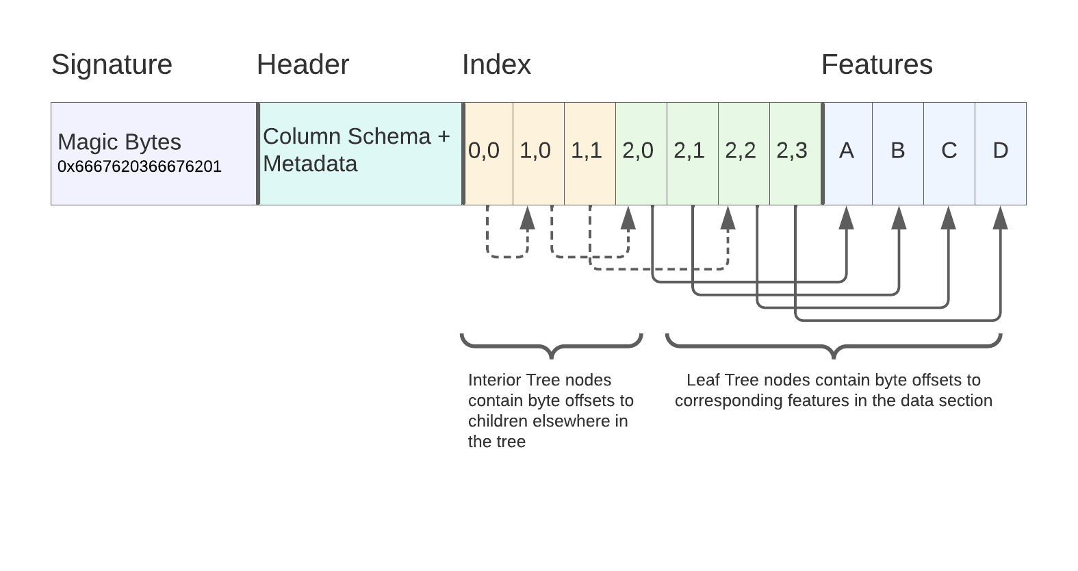
- Signature (static)
- Header (standalone flatbuffer)
- Index – back-to-back index nodes containing bounding boxes and either offsets to other nodes in the tree or to Features in the subsequent data section, depending on whether they are an interior or leaf node
- Features – Back-to-back flatbuffers containing the actual feature data
“Passes” and Buffer Ordering
If you’ve made it this far, you may have noticed that some of the data dependencies between the different sections can pose a few challenges for generating an FGB file.
- Depending on how you derive your column schema, feature count, and envelope for the Header, this likely requires a pass through the feature data to infer.
- To write the Index, you need to first sort, then write, the Features so that you have bounding boxes and known byte offsets for them to include in the Index Nodes
There are a few ways to handle this:
- In memory — If the data you’re writing fits in memory, it’s fairly easy. Buffer it all, do the schema checking and sorting, write additional byte buffers for the Features, then the Header and Index, and finally write it all to a file in the right order
- Partially in memory, with tempfiles — Read features into memory, sort them, write to a tempfile, then build the header and index, then copy all 3 into the final output file. This requires having enough memory to buffer all features in memory and do the sort.
- Partitioned memory with tempfiles — Read sequential feature buffers of a fixed max size, sort each one, record schema and bounding box, then write to a tempfile. Repeat for all features giving N locally-sorted feature tempfiles. Then merge-sort these into a single feature tempfile (will become the “data” section of your final file), recording byte offsets and bounding boxes. Write the Header and Index into the output file then concatenate the Feature section from its tempfile onto the end. I haven’t seen any implementations doing this yet but have been working on it for geoq. This approach should only require enough memory to store the index, which is fairly small. (An FGB index for 1 billion features with node-size of 64 would take 40GB…who knows if this would ever be practical or not)
Most of the implementations I have seen so far use either 1 or 2.